Analyzing Tree Size Structure to Understand
Fire Effects on Population Dynamics
An Introduction to Excel
Synopsis:
Tree diameter measurements reveal the demographic history written into forest stands. They can help us determine whether populations exhibit continuous recruitment or regeneration pulses. In this workshop, you'll learn the ecological theory behind size structure analysis and master Excel techniques to transform DBH data into frequency distributions that expose recruitment bottlenecks and fire effects. Using Caribbean pine data from Belize and your own field measurements, you'll calculate population statistics, create publication-quality graphs, and interpret what different distribution shapes tell us about past disturbance regimes. Students interested in learning these analyses in R programming can download the code and student guide to running R.
In this workshop, you will:
Explore some example data from Belize and perform quality control
Create size class distributions for each treatment
Calculate summary statistics, including mean and standard deviation
Create graphs to compare DBH distributions between treatments
Test whether there are statistical differences between treatments
Interpret results in the context of fire ecology theory
Gain experience using R with the Swirl Package and repeat the Excel activity in R Statistics.

Caribbean Pine (Pinus caribbea)
In collaboration with fire managers in Paynes Creek National Park, Belize, researchers examined the size distribution of 237 Caribbean pine trees. Methods involved sampling six 20×50m plots in 2017, with 3 plots in open savanna environments (low fire intensity, sparse pine canopy, abundant herbaceous cover, little litter) and 3 plots in forest environments (high fire intensity, variable pine overstory, primarily shrub groundcover with some bunchgrasses). Column Definitions:
A: EntryID: Sequential numbers
B: Plot: Plot number (identifies different locations/treatments)
C: Veg: Vegetation/treatment type (savanna and forest)
D: Tag: Individual tree identification number
E: DBH2017: Diameter at breast height in 2017 (cm)
Reference: Fill, J.M., M. Muschamp, F. Tricone, R.M. Crandall, and R. Anderson. 2025. Large trees are most influential for long-term persistence of Caribbean pine (Pinus caribaea var. hondurensis) populations in lowland Belize savannas. Biotropica, DOI: 10.1111/btp.70019.
Data Import
Materials Needed
Files:
CPineData_RawData_forPH.csv (provided)
Excel_Pine_Analysis.xlsx (you'll create this)
Accompanying PowerPoint Presentation (provided)
See here for additional student resources
Software:
Microsoft Excel 2016+ with Analysis ToolPak enabled
To enable the Analysis ToolPak in Excel, go to Home → Add-ins. Search for “Analysis ToolPak'.“ Select “Add.”
Preparation:
Download CPineData_RawData_forPH.csv to your computer
Create a new folder: Caribbean_Pine_Analysis
Save the CSV file in this folder
Import data:
Double-click on the CSV file: CPineData_RawData_forPH.csv
Save your workbook:
File → Save As…
Name it: Caribbean_Pine_Analysis
Select File Format: Excel Workbook (.xlsx)
Save in your Caribbean_Pine_Analysis folder
Rename the sheet:
Right-click on "Sheet1" tab at bottom
Select "Rename"
Type: Raw_Data
Press Enter
MODULE 1: Data Exploration and Quality Control
Part A: Initial Data Exploration
Step 1: Examine the Data
Click on cell A1 (should say "EntryID")
Press Ctrl + Shift + End to jump to the last cell with data
Checkpoint: How many rows are in the dataset?
Step 2: Explore Each Column
Plot Column (Column B):
Click on any cell in column B (e.g., B2)
Insert a PivotTable:
Click Insert tab
Click PivotTable
Select "New Worksheet"
Click OK
In PivotTable Fields pane (See below):
Drag "Plot" to "Rows" box
Drag "Plot" to "Values" box
Click on “Sum of Plot” and select “Count”
Result - This shows you the number of trees per plot. See figure below.
Checkpoint: How many unique trees? Which plot has the highest number of trees
Rename this sheet: Right-click sheet tab → Rename → Plot_Summary
Go back to Raw_Data sheet (click tab at bottom)

Veg Column (Column C):
Click on cell C1
Click Data tab → Filter
Small dropdown arrows appear in each of the header rows
Click the dropdown arrow in "Veg" column
Checkpoint: How many unique values do you see? These are your treatment categories!
DBH2017 Column (Column E):
Click on cell E1
Scroll down to look at the DBH values
Checkpoint: What are the minimum and maximum values? Do you see any unusual values (very small, very large, blank)?
Click Data → Filter again to remove filter (show all data)
MODULE 1: Data Exploration and Quality Control
Part B: Quality Control (QC)Checks
Create a new sheet for organized data:
Click on + at bottom of sheet
Rename it: Organized_Data
Copy data to new sheet:
Go back to Raw_Data sheet
Click cell A1
Press Ctrl + A to select all data
Press Ctrl + C (copy)
Go to Organized_Data sheet
Click cell A1
Press Ctrl + V (paste)
QC Check #1: Missing DBH Values
Click on cell F1 in Organized_Data sheet
Type: QC_Flag
Press Enter
Click on cell F2
Copy-paste or type this formula EXACTLY:
=IF(ISBLANK(E2),"Missing",IF(E2<2,"Too Small",IF(E2>80,"Very Large","OK")))Press Enter
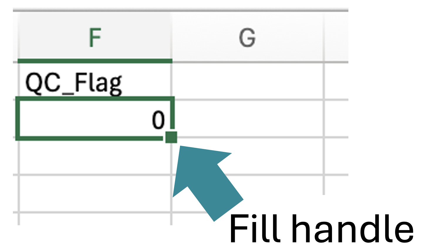
Click back on F2
Double-click the fill handle (small square at bottom-right of cell; see figure below), which will copy formula down to all rows
Click on cell F1 (header)
Click Data → Filter
Click the dropdown in QC_Flag column
Checkpoint: What do you see? Number of "Missing"? Number of "Too Small"? Number of "Very Large"?
QC Check #2: Check Treatment Consistency
Click the dropdown in Veg column. This shows if treatment names are spelled consistently.
Checkpoint: Look at the highlighted cells. Are there variations in spelling or capitalizations (e.g., "Savanna" vs "savanna")? Are there typos? If you find variations, standardize them using Find & Replace
Click Data → Filter again to remove filter (show all data)
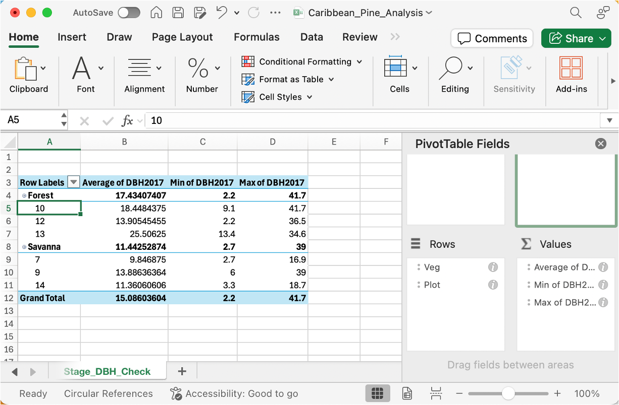
QC Check #3: DBH Range by Life Stage
Create a PivotTable: Select all data - Insert → PivotTable → New Worksheet
Set up the PivotTable:
Drag "Veg" to Rows
Drag “Plot” to Rows
Drag "DBH2017" to Values
Click on "Sum of DBH2017" → Value Field Settings → Average
Drag "DBH2017" to Values again
Click on this second one → Value Field Settings → Min
Drag "DBH2017" to Values a third time
Click on this one → Value Field Settings → Max
Rename this sheet: Stage_DBH_Check
You should see:
MODULE 2: Size Class Distributions
Part A: Set Up Analysis Parameters
Create a new sheet:
Insert new worksheet
Rename: Parameters
Create parameter table:
In the Parameters sheet, create this table starting at A1, adjusting column widths as necessary. Do not enter anything in []:
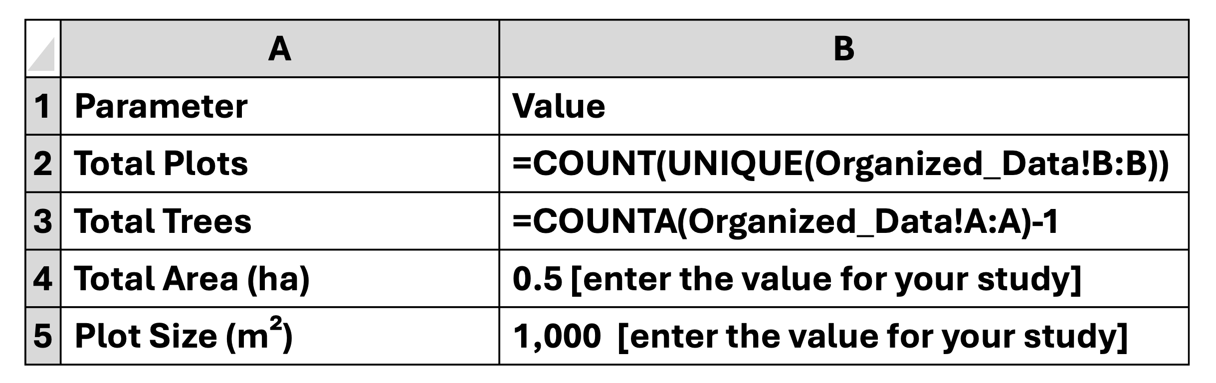
2. Here are the formulas to copy-paste:
=COUNT(UNIQUE(Organized_Data!B:B))
=COUNTA(Organized_Data!A:A)-1
MODULE 2: Size Class Distributions
Part B: Create Size Classes
Go back to Organized_Data sheet
Add Size Class Column:
Click on cell G1
Type: Size_Class
Press Enter
Click on cell G2
Type this formula (this is complex - copy carefully!):
=IF(E2<5,"2-5",IF(E2<10,"5-10",IF(E2<15,"10-15",IF(E2<20,"15-20",IF(E2<25,"20-25",IF(E2<30,"25-30",IF(E2<35,"30-35",IF(E2<40,"35-40",IF(E2<45,"40-45",IF(E2<50,"45-50","50+"))))))))))Press Enter
Click back on G2
Double-click fill handle to copy down.
Checkpoint: Verify it worked: Tree with DBH = 7.5 should show "5-10" Tree with DBH = 23 should show "20-25"Every tree should now have a size class!
MODULE 2: Size Class Distributions
Part C: Calculate Frequency Distributions
Create new sheet:
Insert new worksheet
Rename: Size_Distribution
Step 1: Identify Your Treatments
Go back to Organized_Data sheet
What treatments are in the "Veg" column?
Step 2: Create Frequency Table Structure
In the Size_Distribution sheet:
Row 1 (Headers):
Starting in A1, type these headers (one per column):
A1: Size_Class
B1: Savanna_Count (use YOUR treatment names, e.g., Burned and Unburned instead of Savanna and Forest)
C1: Savanna_%
D1: Forest_Count
E1: Forest_%
(Add more column pairs if you have more treatments)
Column A (Size Classes):
Select entire column and right-click → Select Format Cells → Select Text → Click OK
Starting at A2, type these size classes (one per row):
2-5
5-10
10-15
15-20
20-25
25-30
30-35
35-40
40-45
45-50
50+
Step 3: Count Trees in Each Size Class
CRITICAL: Replace "Savanna" in the formulas below with YOUR actual treatment name from the Veg column!
In cell B2 (count for 2-5 cm, Savanna treatment):
=COUNTIFS(Organized_Data!$C:$C,"Savanna",Organized_Data!$G:$G,"2-5")
Explanation:
Organized_Data!$C:$C = Veg column (treatment)
"Savanna" = name of treatment (CHANGE THIS to your actual treatment name!)
Organized_Data!$G:$G = Size_Class column
"2-5" = size class we're counting
In cell B3 (count for 5-10 cm, Savanna):
=COUNTIFS(Organized_Data!$C:$C,"Savanna",Organized_Data!$G:$G,"5-10")
Continue for ALL size classes (B4 through B12):
Change the last part to match the size class in column A:
B4: 10-15
B5: 15-20
B6: 20-25
B7: 25-30
B8: 30-35
B9: 35-40
B10: 40-45
B11: 45-50
B12: 50+
Repeat for your second treatment (Column D):
In cell D2:
=COUNTIFS(Organized_Data!$C:$C,"Forest",Organized_Data!$G:$G,"2-5")
Continue for D3 through D12, changing "Forest" to YOUR second treatment name.
Step 4: Calculate Percentages
In cell C2:
=B2/SUM($B$2:$B$12)*100
IMPORTANT: The $ signs make the SUM range absolute, so when you copy down, it always sums B2:B12.
Copy this formula down:
Double-click fill handle to copy down
Repeat for your second treatment (Column E):
In cell E2:
=D2/SUM($D$2:$D$12)*100
Double-click fill handle to copy down
Step 5: Add TOTAL row
In A13: Type TOTAL
In B13:
=SUM(B2:B12)
In C13:
=SUM(C2:C12)
In D13:
=SUM(D2:D12)
In E13:
=SUM(E2:E12)
Alternatively, drag the fill handle to the right
Format the TOTAL row:
Select A13:E13
Home → Font → Bold
Home → Font → Borders → Top Border
Checkpoint:
Do your percentages sum to 100%?
Which size class has the most trees in Savanna treatment?
Which size class has the most trees in Forest treatment?
MODULE 3: Summary Statistics and Comparisons
Part A: Calculate Basic Statistics
Create new sheet:
Insert new worksheet
Rename: Summary_Stats
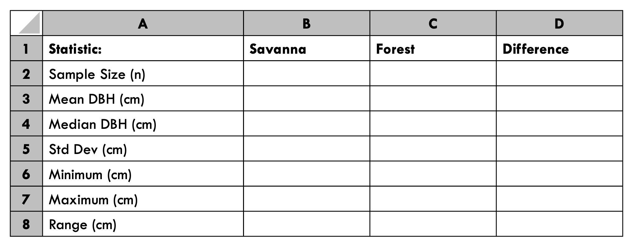
Step 1: Create Statistics Table Structure
Create this table starting at A1:
Step 2: Calculate Statistics for savanna Treatment
IMPORTANT: Change "Savanna" and “Forest” in these formulas to YOUR treatment names!
In B2 (Sample Size):
=COUNTIFS(Organized_Data!$C:$C,"Savanna",Organized_Data!$E:$E,">0")This counts trees in Savanna treatment that have a DBH > 0.
In B3 (Mean):
=AVERAGEIF(Organized_Data!$C:$C,"Savanna",Organized_Data!$E:$E)In B4 (Median):
This requires an array formula:
=MEDIAN(IF(Organized_Data!$C:$C="Savanna",Organized_Data!$E:$E))In B5 (Std Dev):
=STDEV.S(IF(Organized_Data!$C:$C="Savanna",Organized_Data!$E:$E))Press Ctrl + Shift + Enter
In B6 (Minimum):
For Excel 2019+:
=MINIFS(Organized_Data!$E:$E,Organized_Data!$C:$C,"Savanna")In B7 (Maximum):
=MAXIFS(Organized_Data!$E:$E,Organized_Data!$C:$C,"Savanna")In B8 (Range):
=B7-B6Step 3: Repeat for Forest Treatment (Column C)
Copy all formulas from column B to column C, then use Find & Replace:
Select C2:C8
Press Ctrl + H (Find & Replace)
Find: "Savanna"
Replace: "Forest"
Click "Replace All" (There should be 6 replacements)
Step 4: Calculate Differences (Column D)
In D2:
=C2-B2Use fill handle to copy down to D3:D8
MODULE 3: Summary Statistics and Comparisons
Part B: Advanced Statistics
Continue in Summary_Stats sheet
Add a couple more rows below your current table, starting at A9 with DISTRIBUTION METRICS:

6. Calculate Coefficient of Variation (CV) and Skewness
In B10:
=(B5/B3)*100This is: (Std Dev / Mean) × 100
In C10:
=(C5/C3)*100In D10:
=B10-C10Interpretation of CV:
Add a column E for Savanna interpretation and a column F for Forest interpretation:
In E10:
=IF(B10<30,"Low (even-aged)",IF(B10<60,"Moderate","High (uneven-aged)"))Copy to F10 (for Forest interpretation):
=IF(C10<30,"Low (even-aged)",IF(C10<60,"Moderate","High (uneven-aged)"))Row 11: Skewness
Skewness is trickier in Excel without add-ins.
Simple approximation using Pearson's method:
In B11:
=3*(B3-B4)/B5This is: 3 × (Mean - Median) / Std Dev
In C11:
=3*(C3-C4)/C5Interpretation:
Positive skewness (>0.5) = right-skewed, more small trees
Near zero (-0.5 to 0.5) = symmetric
Negative skewness (<-0.5) = left-skewed, more large trees
Add interpretation in E11 for Savanna treatment:
=IF(B11>0.5,"Right-skewed (many small trees)",IF(B11<-0.5,"Left-skewed (many large trees)","Approximately symmetric"))Add interpretation in E12 for Forest treatment:
=IF(C11>0.5,"Right-skewed (many small trees)",IF(C11<-0.5,"Left-skewed (many large trees)","Approximately symmetric"))Checkpoint: Let’s discuss your results so far.
MODULE 4: Create Figures
Figure 1: Size Class Distribution Histogram
Go to Size_Distribution sheet
Select your data for the chart:
Click on cell A1
Drag to select: A1:A12, C1:C12, E1:E12 (We're selecting Size_Class and the two Percent columns)
Hold Ctrl and click to select non-adjacent columns
Insert Chart:
Click Insert tab
Click Insert 2D Column Chart
Select Clustered Column (first option)
A chart appears!
Format the chart:
Chart Title:
Click on title
Type: Size Class Distribution by Treatment
Axis Titles:
Chart Design → Add Chart Element → Axis Titles → Primary Horizontal
Click in text box → Delete “Axis title” → Type: Diameter Class (cm)
Chart Design → Add Chart Element → Axis Titles → Primary Vertical
Click in text box → Delete “Axis title” → Type: Frequency (%)
Go to Home and change font style and size
Remove gaps between bars (make it look like a histogram):
Right-click on any bar
Select Format Data Series
Series Options (bar chart icon)
Gap Width: Move slider to 0%
Color the bars:
Right-click on Savanna bars → Format Data Series
Fill & Border (paint bucket icon)
Fill → Solid fill
Color: Choose a color that represents savannas
Right-click on Forest bars
Choose a color that represents forests
Move legend to top:
Click legend
Chart Design → Add Chart Element → Legend → Top
6. Move chart to its own sheet:
Right-click on chart
Move Chart
Select New sheet
Name: Fig1_SizeDistribution
Click OK
Checkpoint:
Does either treatment show a reverse J-shape?
Which treatment shows a more normal distribution?
What does this tell you about recruitment?
Figure 2: Side-by-Side Comparison of Means
Go to Summary_Stats sheet
Select cells A3:C3 (Mean DBH row with treatments)
Insert → Column Chart → Clustered Column
Format the chart:
Title: Mean DBH by Treatment
Y-axis: Mean DBH (cm)
If there is a legend, remove it (only 2 bars, labels on X-axis are clear)
Add labels to bars
Right-click chart → Select Data
Horizontal Axis Labels → Edit
Select B1:C1 (Savanna, Forest)
Click OK
Add Error Bars (Standard Error):
Click on one bar
Chart Design → Add Chart Element → Error Bars → More Error Bar Options
Error Bar Options:
Direction: Both
End Style: Cap
Error Amount: Custom → Specify Value
Positive Error Value: Select Std Dev for both treatments
Negative Error Value: Same values
Play around with bar colors, fonts, and font sizes
Make bars wider:
Right-click bar → Format Data Series
Change values for Gap Width
MODULE 5: Statistical Tests
Part A: Descriptive Comparison
Create new sheet:
Insert a new worksheet
Rename: Statistical_Tests
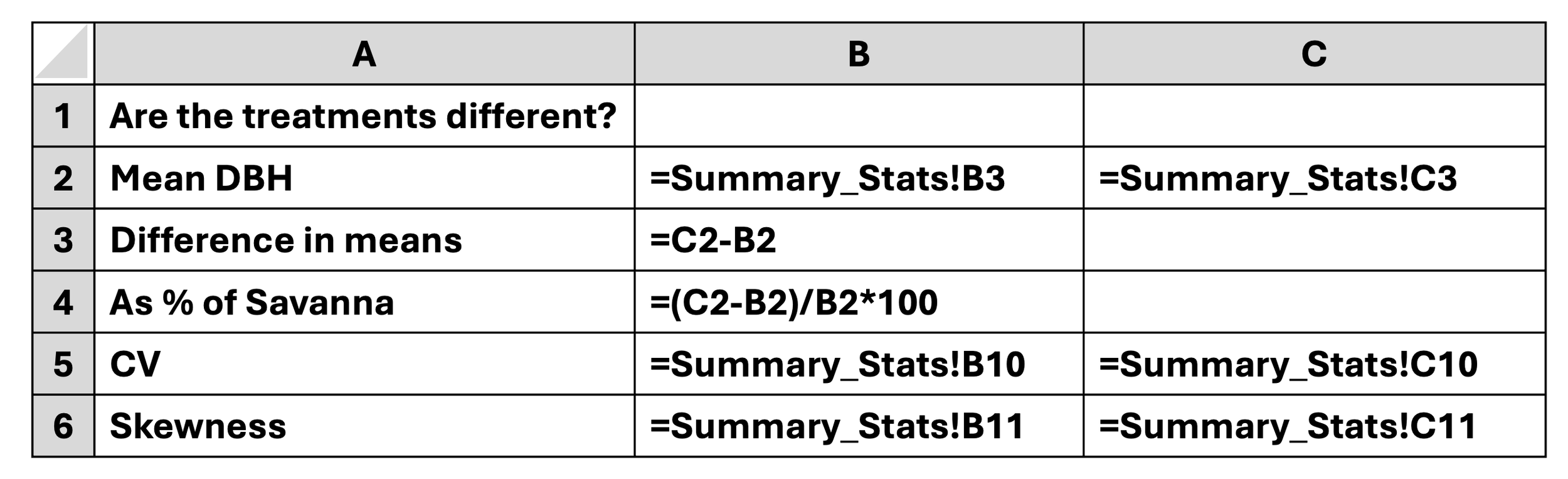
Create a summary comparison:
MODULE 5: Statistical Tests
Part B: F-Test for Equal Variances
This tests if the variability (spread) is different between treatments.
1. In Statistical_Tests sheet, in cell A10, type F-TEST FOR EQUAL VARIANCES
2. Click Data tab → Data Analysis
4. In Data Analysis dialog:
Select F-Test Two-Sample for Variances
Click OK
5. F-Test dialog box:
Variable 1 Range:
Click in the box
Go to Organized_Data sheet
Select the DBH values for savanna: E[first row]:E[last row]
This enters: `Organized_Data!E$137:E$223`
Variable 2 Range:
Click in the box
Go to Organized_Data sheet
Select the DBH values for forest: E[first row]:E[last row]
Labels: Leave unchecked (we didn't select headers)
Alpha: 0.05
Output Range:
Click back on Statistical_Tests sheet
Click cell A12
Click OK
Excel outputs:
F-Test Two-Sample for Variances with various statistics including:
Mean for each variable
Variance for each variable
Observations (number of)
df (degrees of freedom)
F statistic (KEY VALUE)
P(F<=f) one-tail (KEY VALUE)
F Critical one-tail
INTERPRETATION:
In cell C12 (next to output), type: INTERPRETATION
In C13, type:
=IF(B20<0.05,"Variances are SIGNIFICANTLY DIFFERENT (P<0.05)","Variances are EQUAL (P>0.05)")
What it means:
If P < 0.05: Use Welch's t-test (accounts for unequal variances)
If P ≥ 0.05: Use Student's t-test (assumes equal variances)
Checkpoint:
What is the F statistic?
What is the P-value?
Are the variances equal or different?
MODULE 5: Statistical Tests
Part C: T-Test for Mean Difference
This tests if mean DBH is significantly different between treatments.
1. In Statistical_Tests sheet, go to cell A25:
Type: T-TEST FOR MEAN DBH
2. Click Data → Data Analysis → t-Test
Which t-test to choose?
If F-test P < 0.05: t-Test: Two-Sample Assuming Unequal Variances
If F-test P ≥ 0.05: t-Test: Two-Sample Assuming Equal Variances
3. Click OK
4. T-Test dialog:
Variable 1 Range:
Go to Organized_Data sheet
Select DBH values for savanna data
Variable 2 Range:
Go to Organized_Data sheet
Select DBH values for forest data
Hypothesized Mean Difference: 0
Labels: Unchecked
Alpha: 0.05
Output Range: Cell A27 in Statistical_Tests sheet
5. Click OK
Excel outputs:
t-Test results including:
Mean for each variable
Variance for each variable
Observations
df (degrees of freedom) - KEY
t Stat (KEY VALUE)
P(T<=t) one-tail
t Critical one-tail
P(T<=t) two-tail (KEY VALUE - use this one!)
t Critical two-tail
INTERPRETATION:
Add interpretation next to output:
In column C next to the t-test output:
Label cell (e.g., E27): INTERPRETATION
Next cell (e.g., E28):
=IF(B38<0.001,"Means are HIGHLY SIGNIFICANTLY DIFFERENT (P<0.001)",IF(B38<0.01,"Means are SIGNIFICANTLY DIFFERENT (P<0.01)",IF(B38<0.05,"Means are SIGNIFICANTLY DIFFERENT (P<0.05)","Means are NOT significantly different (P>0.05)")))
2. Write your statistical statement:
In cell A40:
="Mean DBH was "&IF(B38<0.05,"significantly ","not significantly ")&"different between treatments (Savanna: "&TEXT(Summary_Stats!B3,"0.0")&" cm, Forest: "&TEXT(Summary_Stats!C3,"0.0")&" cm; t="&TEXT(B35,"0.00")&", df="&TEXT(B34,"0")&", P="&TEXT(B38,"0.000")&")."
This automatically generates a results sentence!
Checkpoint:
What is the t-statistic?
What are the degrees of freedom (i.e., df)?
What is the P-value (two-tailed)?
Are the means significantly different?
MODULE 6: Interpretation Questions
Size Structure: Which treatment has higher CV? What does this indicate about age structure?
Distribution Shape: Which treatment is right-skewed (positive skewness)? What does this mean ecologically? Is this what you'd expect based on the lecture?
Statistical Significance: Are the means significantly different? Is this difference large enough to be ecologically important?
Fire Trap Evidence: Do you see a "missing middle" in any treatment? Which size classes are under-represented? What does this suggest about fire effects?
Discussion questions
Did your results match the predictions from the lecture? Why or why not?
What ecological processes explain the patterns you observed?
What are the management implications of these findings?
MODULE 7: An introduction to R Programming
Swirl is an R package designed to teach R programming and data science interactively within the R console. It provides a series of courses and lessons that guide users through various R concepts and functionalities, and offers a hands-on and interactive way for beginners to learn R programming by practicing directly within the R environment
Using Swirl for R beginners:
Install R and RStudio: Ensure you have R (version 3.1.0 or later) and RStudio (recommended for a better experience) installed on your computer.
Install the Swirl package: Open RStudio and type the following command in the console:
install.packages("swirl")
Load the Swirl package: Load the package into your R session:
library(swirl)
Start Swirl: Initiate the Swirl environment:
swirl()You will be prompted to enter your name, which allows Swirl to track your progress.
Install a course: The first time you run Swirl, you'll be prompted to install a course. You can choose from recommended courses or explore the Swirl Course Network for more options. For example, to install the "R Programming" course
install_course("R Programming")
Note: Course names are case-sensitive.
Select a lesson:
After installing a course, you can choose a specific lesson to begin. Swirl will present a menu of available lessons. It is recommended that you start with “1: R Programming: The basics of programming in R.”
Engage with the interactive lessons:
Swirl will guide you through the lesson with text explanations, questions, and prompts to enter R code directly into the console.
Press Enter when you see ... to continue reading.
Type your responses or R code when you see the R prompt (>) or a specific prompt from Swirl.
Swirl provides immediate feedback on your code and answers.
Helpful commands within Swirl:
bye(): Exit Swirl and save your progress.
skip(): Skip the current question.
play(): Temporarily exit Swirl to experiment with R in the console.
next(): Regain Swirl's attention after using play().
main(): Return to the main Swirl menu.
info(): Display options and instructions again.
Once you are comfortable with R, you can try replicating the Excel activity from above using this R code and the associated student guide to running R code.